Preprocessing

Import and wrangle mutlisourced influenza observations

Preliminaries

Setup working environment and loading necessary packages.

Libraries

Hide code

#wrangling
library(tidyverse)
library(lubridate)
library(data.table, include.only = "fread")
library(cdcfluview)
library(yaml)

#spatial
library(sp)
library(sf)
library(spdep)
library(rgeos)
library(igraph)
library(maptools)
library(mapproj)
library(CovidCAR)
#devtools::install_github("JMHumphreys/CovidCAR")

#messages
library(cli)

#inference
library(INLA)

#Utilities
#source("./R/utilities.R")

options(dplyr.summarise.inform = FALSE)

#function
download_file <- function(url, filename) {
  download.file(url, destfile = filename, method = "auto", quiet = FALSE, mode = "wb")
}

Observation Data

FluSurv

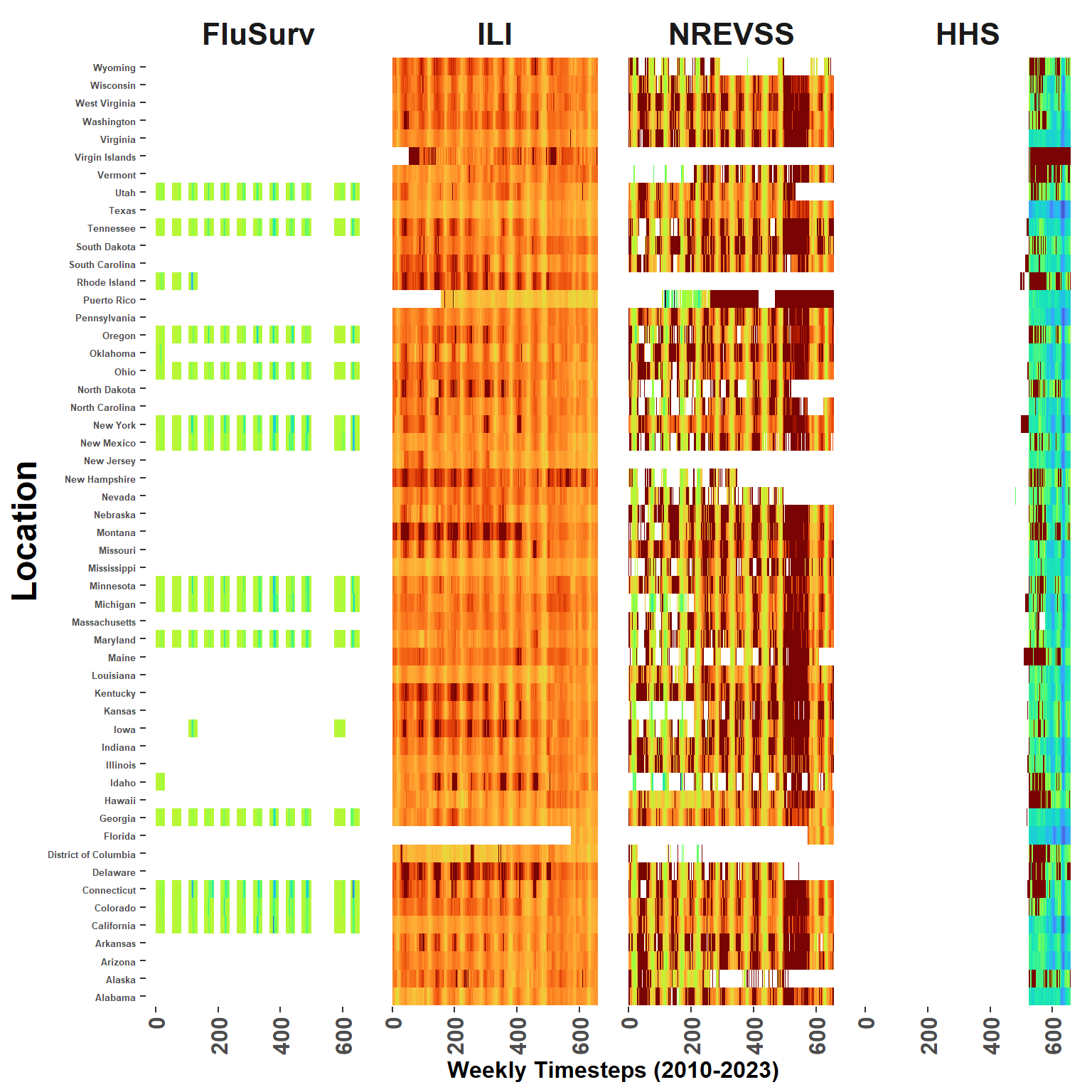
Build a flu hospitalization data file from individual state reports and all available years. The hospitalizations() function from the cdcfluview package does most of the work by querying FluView, but seems only to be able to take small bites at a time.

Hide code

myRegions <- surveillance_areas() 

flusurv_all <- do.call(rbind, lapply(seq_len(dim(myRegions)[1]), function(i) {
  hospitalizations(surveillance_area = myRegions$surveillance_area[i], region = myRegions$region[i])
}))

Wrangle Flusurv data:
Note that the cdcfluview package only includes through Spring of 2020. Because of this, the data is filtered at 2019 and a static file manually downloaded from FluView with more recnt reports (eventually this data will be moved to www.healthdata.gov).

Hide code

range(flusurv_all$year)

[1] 2003 2020

Hide code

flusurv <- flusurv_all %>%
  filter(age_label == "Overall",
         region != "Entire Network",
         year >= 2010 & year <= 2019) %>% #the pkg fails on dates after 2020,ugh
  mutate(location_name = region,
         network = surveillance_area,
         weeklyrate = as.numeric(weeklyrate),
         epiweek = year_wk_num) %>%
    select(location_name, year, epiweek, network, rate, weeklyrate)
  
#manual download from site 2023-06-01
flusurv_2020 <- fread("D:/Github/flusion/data/FluSurveillance_2020.csv") %>%
  rename_all(~gsub(" |-", "", .)) %>%
  filter(AGECATEGORY == "Overall",
         SEXCATEGORY == "Overall",
         RACECATEGORY == "Overall",
         CATCHMENT != "Entire Network",
         MMWRYEAR >= 2020) %>% #Prior to this date was downloaded in code above
  mutate(location_name = CATCHMENT,
         network = NETWORK,
         year = MMWRYEAR,
         epiweek = MMWRWEEK,
         rate = CUMULATIVERATE,
         weeklyrate = as.numeric(WEEKLYRATE)) %>%
    select(location_name, year, epiweek, network, rate, weeklyrate)

#Join date ranges and scale weeklyrate
flusurv = rbind(flusurv, flusurv_2020)
flusurv$weeklyrate.s = as.numeric(scale(flusurv$weeklyrate, scale = T, center=T))

#combine NY data
flusurv$location_name[flusurv$location_name == "New York - Albany"] = "New York"
flusurv$location_name[flusurv$location_name == "New York - Rochester"] ="New York"

flusurv <- flusurv %>%
  group_by(location_name, year, epiweek) %>%
  summarise(rate = mean(rate, na.rm=T),
            weeklyrate = mean(weeklyrate, na.rm=T),
            weeklyrate.s = mean(weeklyrate.s, na.rm=T))


#Check for duplicates
unique(duplicated(flusurv))

[1] FALSE

Hide code

dim(flusurv)

[1] 5676    6

Hide code

head(flusurv)

location_name	year	epiweek	rate	weeklyrate	weeklyrate.s
California	2010	1	NA	0.4	-0.4771582
California	2010	2	NA	0.2	-0.5561987
California	2010	3	NA	0.2	-0.5561987
California	2010	4	NA	0.2	-0.5561987
California	2010	5	NA	0.2	-0.5561987
California	2010	6	NA	0.1	-0.5957189

Same FluSurv process as above, but now for the Full Network reports

Hide code

flusurv_en <- flusurv_all %>%
  filter(age_label == "Overall",
         region == "Entire Network",
         year >= 2010 & year <= 2019) %>% #the pkg fails on dates after 2020,ugh
  mutate(location_name = region,
         network = surveillance_area,
         epiweek = year_wk_num) %>%
    select(location_name, year, epiweek, network, rate, weeklyrate)

flusurv_en2020 <- fread("D:/Github/flusion/data/FluSurveillance_2020.csv") %>%
  rename_all(~gsub(" |-", "", .)) %>%
  filter(AGECATEGORY == "Overall",
         SEXCATEGORY == "Overall",
         RACECATEGORY == "Overall",
         CATCHMENT == "Entire Network",
         MMWRYEAR >= 2020) %>% #the pkg fails on dates after 2020,ugh
  mutate(location_name = CATCHMENT,
         network = NETWORK,
         year = MMWRYEAR,
         epiweek = MMWRWEEK,
         rate = CUMULATIVERATE,
         weeklyrate = WEEKLYRATE) %>%
    select(location_name, year, epiweek, network, rate, weeklyrate)

#Join
flusurv_en <- rbind(flusurv_en, flusurv_en2020)
unique(duplicated(flusurv_en))

[1] FALSE

Hide code

dim(flusurv_en)

[1] 1131    6

Hide code

head(flusurv_en)

location_name	year	epiweek	network	rate	weeklyrate
Entire Network	2016	40	FluSurv-NET	0.1	0.1
Entire Network	2016	41	FluSurv-NET	0.2	0.1
Entire Network	2016	42	FluSurv-NET	0.3	0.1
Entire Network	2016	43	FluSurv-NET	0.4	0.1
Entire Network	2016	44	FluSurv-NET	0.6	0.1
Entire Network	2016	45	FluSurv-NET	0.8	0.2

ILINet Surveillance Data

Influenza Like Illness (ILI) data using cdcfluview package. Unlike FluSurv, data is available 2010-2013.

Hide code

ilinet <- ilinet(region = "state") %>%
  mutate(location_name = region,
         epiweek = week,
         unweighted = as.numeric(unweighted_ili),
         unweighted.s = unweighted,
         total = ilitotal,
         providers = num_of_providers) %>%
  select(location_name, year, epiweek, unweighted, unweighted.s, total, providers)

# Clip to between 0.0001 and 99.999
ilinet$unweighted.s <- pmin(pmax(as.numeric(ilinet$unweighted.s), 0.01), 99.99)/100

# logit transform 
ilinet$unweighted.s <- log(ilinet$unweighted.s/(1-ilinet$unweighted.s))
range(ilinet$unweighted.s, na.rm=T)

[1] -9.210240 -1.423094

Hide code

unique(duplicated(ilinet))

[1] FALSE

Hide code

dim(ilinet)

[1] 35678     7

Hide code

range(ilinet$year)

[1] 2010 2023

Hide code

head(ilinet)

location_name	year	epiweek	unweighted	unweighted.s	total	providers
Alabama	2010	40	2.134770	-3.825232	249	35
Alaska	2010	40	0.875146	-4.729745	15	7
Arizona	2010	40	0.674721	-4.991856	172	49
Arkansas	2010	40	0.696056	-4.960510	18	15
California	2010	40	1.954120	-3.915496	632	112
Colorado	2010	40	0.660684	-5.013021	134	14

COVID19 RPIHC

Downloading the COVID-19 Reported Patient Impact and Hospital Capacity by State Timeseries from https://healthdata.gov/.

Hide code

url <- "https://healthdata.gov/api/views/g62h-syeh/rows.csv?accessType=DOWNLOAD"
filename <- "D:/Github/flusion/data/flu_HHS.csv"

download_file(url, filename)

Read and wrangle RPIHC:

Hide code

flu_HHS <- fread("D:/Github/flusion/data/flu_HHS.csv") %>%
  mutate(abbreviation = state,
         date = as_date(date) - 1, #1-day prior, per fluSight truth
         year = year(date),
         epiweek = epiweek(date)) %>%
  group_by(abbreviation, year, epiweek) %>%
  summarise(hosp_inc = sum(previous_day_admission_influenza_confirmed))

unique(duplicated(flu_HHS))

[1] FALSE

Hide code

dim(flu_HHS)

[1] 9346    4

Hide code

range(flu_HHS$year)

[1] 2019 2023

Hide code

head(flu_HHS)

abbreviation	year	epiweek	hosp_inc
AK	2020	13	NA
AK	2020	14	NA
AK	2020	15	NA
AK	2020	16	NA
AK	2020	17	NA
AK	2020	18	NA

NREVSS

National Respiratory and Enteric Virus Surveillance System.

Again, unfortunately only available through a manual: https://gis.cdc.gov/grasp/fluview/fluportaldashboard.html
Files illustrated here were downloaded on June 2, 2023.

Hide code

nrevss.1 <- fread("D:/Github/flusion/data/WHO_NREVSS_Combined_prior_to_2015_16.csv") %>%
  rename_all(~gsub(" |-", "", .)) %>%
  mutate(location_name = REGION,
         year = YEAR,
         epiweek = WEEK,
         tot_perc = as.numeric(PERCENTPOSITIVE),
         Bpos = as.numeric(B),
         tot_samp = as.numeric(TOTALSPECIMENS),
         Apos = tot_perc - ((Bpos/tot_samp)*100)) %>%
  select(location_name, year, epiweek, Apos)


nrevss.2 <- fread("D:/Github/flusion/data/WHO_NREVSS_Clinical_Labs.csv") %>%
  rename_all(~gsub(" |-", "", .)) %>%
  mutate(location_name = REGION,
         year = YEAR,
         epiweek = WEEK,
         Apos = PERCENTA) %>%
  select(location_name, year, epiweek, Apos) #Apos = Influenza A positive

# Combine 
nrevss <- rbind(nrevss.1, nrevss.2)

# Replace "X" 
nrevss$Apos[nrevss$Apos == "X"] <- NA

# Clip to between 0.0001 and 99.999
nrevss$Apos <- pmin(pmax(as.numeric(nrevss$Apos), 0.01), 99.99)/100

# logit transform 
nrevss$Apos.s <- log(nrevss$Apos/(1-nrevss$Apos))
unique(duplicated(nrevss))

[1] FALSE

Hide code

head(nrevss)

location_name	year	epiweek	Apos	Apos.s
Alabama	2010	40	0.0001000	-9.210240
Alaska	2010	40	0.0001000	-9.210240
Arizona	2010	40	0.0250000	-3.663562
Arkansas	2010	40	0.0001000	-9.210240
California	2010	40	0.0273355	-3.571852
Colorado	2010	40	0.0079000	-4.832961

Location Template

Location Table

Location codes and population numbers from FluSight. Should really get varying census over time period, but these are a start.

Hide code

url <- "https://github.com/cdcepi/Flusight-forecast-data/raw/master/data-locations/locations.csv"
filename <- "D:/Github/flusion/data/locations.csv"

download_file(url, filename)

Read locations:

Hide code

locations <- fread("D:/Github/flusion/data/locations.csv") %>%
  select(-c(count_rate1per100k, count_rate2per100k)) %>%
  filter(location_name != "US") #remove aggregate group

head(locations)

abbreviation	location	location_name	population
AL	01	Alabama	5039877
AK	02	Alaska	732673
AZ	04	Arizona	7276316
AR	05	Arkansas	3025891
CA	06	California	39237836
CO	08	Colorado	5812069

Template

Ensure all locations and times are represented in the analysis. Missing data are plugged with NA.

Dates and Locations

Hide code

myYears <- seq(2010, 2023, by = 1)
week_nums <- 1:52

year_set <- lapply(myYears, function(year) {
  tmp_frame <- locations %>% mutate(year = year)
  
  weekly_set <- lapply(week_nums, function(week_num) {
    tmp_frame_wk <- tmp_frame %>% mutate(epiweek = week_num)
    return(tmp_frame_wk)
  })
  
  weekly_set <- do.call(rbind, weekly_set)
  return(weekly_set)
})

template <- do.call(rbind, year_set)

dim(template)

[1] 38584     6

Hide code

head(template) #all states and times represented

abbreviation	location	location_name	population	year	epiweek
AL	01	Alabama	5039877	2010	1
AK	02	Alaska	732673	2010	1
AZ	04	Arizona	7276316	2010	1
AR	05	Arkansas	3025891	2010	1
CA	06	California	39237836	2010	1
CO	08	Colorado	5812069	2010	1

Hide code

first_record <- min(subset(nrevss, year == 2010)$epiweek) #drop before nrevss data was collected
template$drop_old <- ifelse(template$year == 2010 & template$epiweek < first_record, "drop", "keep")

#most_recent <- max(subset(flu_HHS, year == 2023)$epiweek) #drop future dates
most_recent <- 22 #date available when model run
template$drop_new <- ifelse(template$year == 2023 & template$epiweek > most_recent, "drop", "keep")

template <- template %>% 
  filter(drop_old == "keep" &
         drop_new == "keep") %>%
  select(-c(drop_old, drop_new))

unique(duplicated(template))

[1] FALSE

Time Steps

An index with sequential timesteps.

Hide code

template <- template %>%
  arrange(year, epiweek) %>%
  mutate(ts_week = as.integer(as.factor(year + (epiweek/53))))


range(template$ts_week) #number of epiweeks

[1]   1 659

Spatial Domian

Need to setup directories to use CovidCAR functions. Values here are arbitrary (need to add option to bypass to CovidCAR)

Hide code

setup_analysis(report_date = "2010-01-01", 
               training_period = 2*28, #days
               forecast_horizon = 28, #days
               output_dir = "D:/Github/flusion/data"
)

Get Geographic Boundaries

Hide code

States <- download_boundaries(unit = "state")

Reading layer `us-state-boundaries' from data source 
  `D:\Github\flusion\data\2010-01-01-CovidCAR-run2023-06-14\polygons' 
  using driver `ESRI Shapefile'
Simple feature collection with 56 features and 20 fields
Geometry type: MULTIPOLYGON
Dimension:     XY
Bounding box:  xmin: -179.2311 ymin: -14.60181 xmax: 179.8597 ymax: 71.44069
Geodetic CRS:  WGS 84

Hide code

class(States)

[1] "SpatialPolygonsDataFrame"
attr(,"package")
[1] "sp"

Hide code

head(States@data[,c("Region", "State")]) #appended attributes  

Region	State
1	Virgin Islands
2	Wisconsin
3	Vermont
4	New Jersey
5	Colorado
6	South Carolina

Adjacency

Hide code

nb_flusion = get_neighbors(States, connect=TRUE)
summary(nb_flusion)

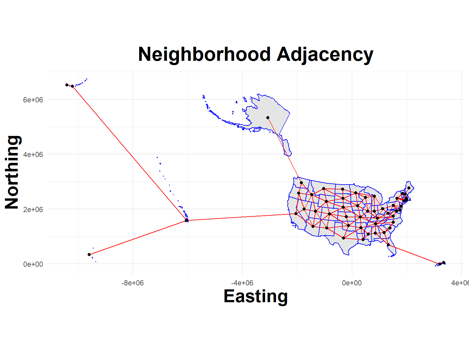
Neighbour list object:
Number of regions: 56 
Number of nonzero links: 242 
Percentage nonzero weights: 7.716837 
Average number of links: 4.321429 
Link number distribution:

 1  2  3  4  5  6  7  8 
 5  3 10 12 10 11  3  2 
5 least connected regions:
1 13 38 42 54 with 1 link
2 most connected regions:
49 56 with 8 links

Hide code

#view
plot_neighbors(States, nb_flusion)

Hide code

#convert to matrix
nb2INLA("J", nb_flusion)
J = inla.read.graph("J")

Template Spatial Index

Hide code

template$Region =  with(States@data[,c("Region", "State")],
                       Region[match(
                        template$location_name,
                                 State)])

Add Entire Network

Getting the flue weeklyrate from FluSurv. Not that this is only the time trend from FluSurv and is not loaction specific.

Hide code

en_match <- flusurv_en %>%
  group_by(year, epiweek) %>%
  summarise(en_est = mean(as.numeric(weeklyrate), na.rm=TRUE)) %>%
  select(year, epiweek, en_est)

# Clip to between 0.0001 and 99.999
en_match$en_est.s <- pmin(pmax(as.numeric(en_match$en_est), 0.01), 99.99)/100

# logit transform 
en_match$en_est.s <- round(log(en_match$en_est.s/(1-en_match$en_est.s)), 3)
range(en_match$en_est.s, na.rm=T)

[1] -9.21 -2.19

Hide code

template <- left_join(template, en_match, by = c("year", "epiweek"))
unique(duplicated(template))

[1] FALSE

Space-Time Interaction Index

All location-time combinations.

Hide code

template$st_int <- as.integer(as.factor(paste0(template$Region, ".", template$ts_week)))
range(template$st_int)

[1]     1 34927

Join to Disease Data

Join observation data to the template. Times and locations without observations are coded as NA.

Hide code

#FluSurv
flusurv_full <- left_join(template, flusurv, by = c("location_name", "year", "epiweek")) 
flusurv_full$network[is.na(flusurv_full$network)] = "none"
unique(duplicated(flusurv_full))

[1] FALSE

Hide code

head(flusurv_full) #times and locations w/out values assigned NA

abbreviation	location	location_name	population	year	epiweek	ts_week	Region	en_est	en_est.s	st_int	rate	weeklyrate	weeklyrate.s	network
AL	01	Alabama	5039877	2010	40	1	21	0.0333333	-8.006	8568	NA	NA	NA	NA
AK	02	Alaska	732673	2010	40	1	38	0.0333333	-8.006	19771	NA	NA	NA	NA
AZ	04	Arizona	7276316	2010	40	1	11	0.0333333	-8.006	1319	NA	NA	NA	NA
AR	05	Arkansas	3025891	2010	40	1	34	0.0333333	-8.006	17135	NA	NA	NA	NA
CA	06	California	39237836	2010	40	1	47	0.0333333	-8.006	25702	NA	0.1	-0.5957189	NA
CO	08	Colorado	5812069	2010	40	1	5	0.0333333	-8.006	27679	NA	0.1	-0.5957189	NA

Hide code

#ILI Surveillance
ilinet_full <- left_join(template, ilinet, by = c("location_name", "year", "epiweek"))
unique(duplicated(ilinet_full))

[1] FALSE

Hide code

head(ilinet_full)

abbreviation	location	location_name	population	year	epiweek	ts_week	Region	en_est	en_est.s	st_int	unweighted	unweighted.s	total	providers
AL	01	Alabama	5039877	2010	40	1	21	0.0333333	-8.006	8568	2.134770	-3.825232	249	35
AK	02	Alaska	732673	2010	40	1	38	0.0333333	-8.006	19771	0.875146	-4.729745	15	7
AZ	04	Arizona	7276316	2010	40	1	11	0.0333333	-8.006	1319	0.674721	-4.991856	172	49
AR	05	Arkansas	3025891	2010	40	1	34	0.0333333	-8.006	17135	0.696056	-4.960510	18	15
CA	06	California	39237836	2010	40	1	47	0.0333333	-8.006	25702	1.954120	-3.915496	632	112
CO	08	Colorado	5812069	2010	40	1	5	0.0333333	-8.006	27679	0.660684	-5.013021	134	14

Hide code

#HHS 
flu_HHS_full <- left_join(template, flu_HHS, by = c("abbreviation", "year", "epiweek"))
unique(duplicated(flu_HHS_full))

[1] FALSE

Hide code

unique(duplicated(flu_HHS_full[,c("ts_week", "Region")]))

[1] FALSE

Hide code

head(flu_HHS_full)

abbreviation	location	location_name	population	year	epiweek	ts_week	Region	en_est	en_est.s	st_int	hosp_inc
AL	01	Alabama	5039877	2010	40	1	21	0.0333333	-8.006	8568	NA
AK	02	Alaska	732673	2010	40	1	38	0.0333333	-8.006	19771	NA
AZ	04	Arizona	7276316	2010	40	1	11	0.0333333	-8.006	1319	NA
AR	05	Arkansas	3025891	2010	40	1	34	0.0333333	-8.006	17135	NA
CA	06	California	39237836	2010	40	1	47	0.0333333	-8.006	25702	NA
CO	08	Colorado	5812069	2010	40	1	5	0.0333333	-8.006	27679	NA

Hide code

#nrevss 
nrevss_full <- left_join(template, nrevss, by = c("location_name", "year", "epiweek"))
unique(duplicated(nrevss_full))

[1] FALSE

Hide code

head(nrevss_full)

abbreviation	location	location_name	population	year	epiweek	ts_week	Region	en_est	en_est.s	st_int	Apos	Apos.s
AL	01	Alabama	5039877	2010	40	1	21	0.0333333	-8.006	8568	0.0001000	-9.210240
AK	02	Alaska	732673	2010	40	1	38	0.0333333	-8.006	19771	0.0001000	-9.210240
AZ	04	Arizona	7276316	2010	40	1	11	0.0333333	-8.006	1319	0.0250000	-3.663562
AR	05	Arkansas	3025891	2010	40	1	34	0.0333333	-8.006	17135	0.0001000	-9.210240
CA	06	California	39237836	2010	40	1	47	0.0333333	-8.006	25702	0.0273355	-3.571852
CO	08	Colorado	5812069	2010	40	1	5	0.0333333	-8.006	27679	0.0079000	-4.832961

View Coverage

Looking at holes in the data. Not interested in exact values, only comparing data coverage.

Hide code

fs_plt <- flusurv_full %>% 
  mutate(value = weeklyrate.s,
         set = "FluSurv") %>%
  select(location_name, ts_week, value, set)

ili_plt <- ilinet_full %>% 
  mutate(value = unweighted.s,
          set = "ILI") %>%
  select(location_name, ts_week, value, set)

hhs_plt <- flu_HHS_full %>% 
  mutate(value = log(hosp_inc+0.0001),
          set = "HHS") %>%
  select(location_name, ts_week, value, set)

nrevss_plt <- nrevss_full %>% 
  mutate(value = Apos.s,
          set = "NREVSS") %>%
  select(location_name, ts_week, value, set)


all_plts <- rbind(fs_plt, ili_plt, hhs_plt, nrevss_plt)
all_plts$set <- ordered(factor(all_plts$set), levels = c("FluSurv", "ILI", "NREVSS", "HHS"))

ggplot() +
geom_tile(data=all_plts,
          aes(ts_week, location_name, fill = value)) +
xlab(" ") +
viridis::scale_fill_viridis(paste0(" "),
                             discrete=F,
                             option = "turbo",
                             direction = -1,
                             na.value = "white") +
ylab("Location") +
xlab("Weekly Timesteps (2010-2023)") +
facet_wrap(~set, ncol = 4) +
theme(panel.grid.minor = element_blank(),
      panel.grid.major = element_blank(),
      panel.background = element_blank(),
      plot.background = element_blank(),
      panel.border = element_blank(),
      legend.title = element_text(size = 16, face = "bold", hjust=0.5),
      legend.text = element_text(size=10, face="bold"),
      strip.text = element_text(size=16, face="bold"),
      strip.background = element_blank(),
      legend.position="none", 
      legend.direction = "horizontal",
      legend.box = "horizontal",
      axis.text.y = element_text(face="bold", size=5),
      axis.text.x = element_text(face="bold", size=12, vjust=0.5,
                                 hjust=1, angle=90),
      axis.title.x = element_text(size=12, face="bold"),
      axis.title.y = element_text(size=18, face="bold"),
      plot.title = element_text(size=18, face="bold", hjust=0.5)) +
guides(color = guide_legend(title.position = "top", label.position = "bottom"))